Ordinary differential equations of 1-st order
Initial (Cauchy) problem for one equation: y ' = f(x,y)
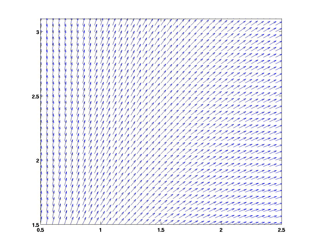
Visualization of all solutions of the equation using direction field
Example: Visualize direction field of the equation y ' = y / x2 on a rectangular domain [ 0.8 , 2.5 ] x [ 0.8 , 3.8 ] :
>> h = 0.1;                          % step-size of the mesh
>> xh = 0.8 : h : 2.5 ;              % xh is the interval [ 0.8 , 2.5 ] divided with step h
>> yh = 0.8 : h : 3.8 ;              % yh  is the interval [ 0.8 , 3.8 ] divided with step h
>> [xx,yy] = meshgrid(xh,yh);        % mesh on the rectangle [ 0.8 , 2.5 ] x [ 0.8 , 3.8 ]
>> px = ones(length(yh),length(xh)); % px = 1 at every mesh-point [x,y]
>> py = yy./xx.^2;                   % py = f(x,y) at every mesh-point [x,y]
>> pp = sqrt(px.*px + py.*py);
>> ppx = px./pp;                     % (ppx, ppy) = normalized (px, py)
>> ppy = py./pp;
>> quiver(xh, yh, ppx, ppy)          % depicts (ppx, ppy) at every [x,y] by an arrow
>> axis equal                        % sets length of x-units equal to y-units
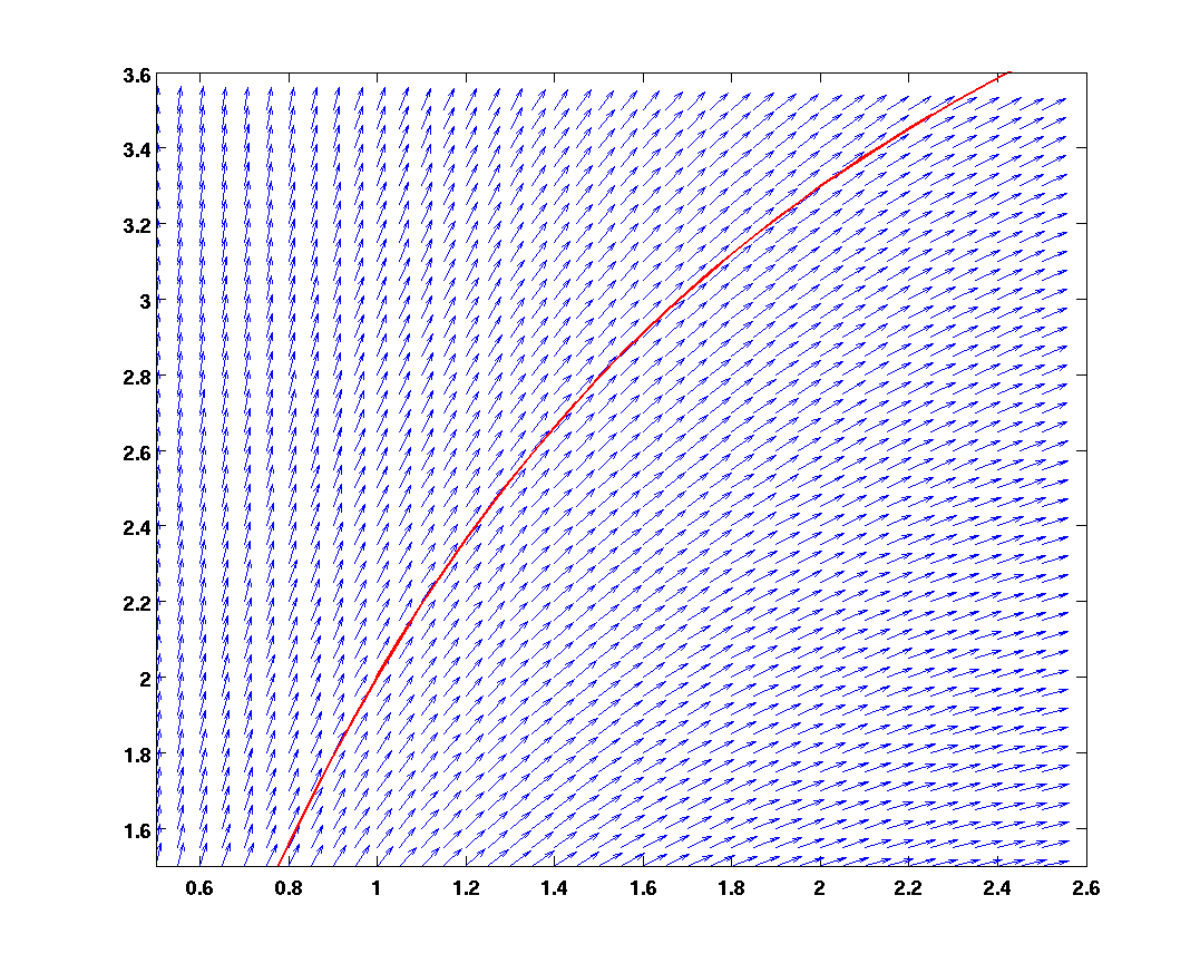
Add to the previous figure the exact solution of y ' = y / x2 for the initial condition y(1) = 2, as a red curve:
>> hold on                           % continue at the same figure
>> plot(xh, 2*exp(1-1./xh),'LineWidth',2,'Color','r')   % exact solution
>> axis([0.5, 2.6, 1.5, 3.6])        % setting a scope
Numerical solution of a Cauchy problem y ' = f(x,y), y(x0) = y0
Solve the equation numerically with step h = 0.2 using Euler and Collatz methods.
>> h = 0.2;          % step-size
>> x = 1; y = 2;     % initial condition - starting point
>> hold on           % use the same figure
>> plot(x, y, 'r*')  % depict starting point as a red asterisk
Explicit Euler's method
Repeat the following 4 steps:
>> f = y / x^2;      % f ... direction of the tangent line at [x, y]
>> x = x + h;        % new value of x
>> y = y + f * h;    % new value of y (on the tangent line)
>> plot(x, y, 'r*')  % plotting the new point
Collatz method
>> x = 1; y = 2; % initial condition - starting point
Repeat the following steps:
>> f = y / x^2;            % f ... direction of the tangent line at [x, y]
>> xp = x + 0.5 * h;       % auxiliary point [xp, yp]
>> yp = y + 0.5 * f * h;   %   (computed by Euler method with half step)
>> fp = yp / xp^2;         % fp ... direction of the tangent line at [xp, yp]
>> x = x + h;              % new value of x
>> y = y + fp * h;         % new value of y (on the tangent line at [xp, yp])
>> plot(x, y, 'b*')        % plotting the new point
Implicit Euler's method
>> x = 1; y = 2; % initial condition - starting point
Repeat the following 4 steps:
>> x = x + h;          % new value of x
>> y = y*x^2/(x^2- h); % new value of y (formula must be tailored for a given equation)
>> plot(x, y, 'g*')    % plotting the new point
Runge-Kutta RK4 method
The following program is for illustration only, how the RK4 works. In practice you should use Matlab function ODE45.
>> x = 1; y = 2; % initial condition - starting point
Repeat the following steps:
>> k1 = y / x^2;           % k1 ... direction of the tangent line at [x, y]
>> xp = x + 0.5 * h;       % trial point [xp, yp]
>> yp = y + 0.5 * k1 * h;  %   (computed by Euler method with half step)
>> k2 = yp / xp^2;         % k2 ... direction of the tangent line at [xp, yp]

>> yq = y + 0.5 * k2 * h;  % second trial point [xp, yq]
>> k3 = yq / xp^2;         % k3 ... direction of the tangent line at [xp, yq]

>> x = x + h;              % new value of x
>> ye = y + k3 * h;        % third trial point [x, ye]
>> k4 = ye / x^2;          % k4 ... direction of the tangent line at [x, ye]

>> y = y + (k1 + 2*k2 + 2*k3 + k4) * h/6;  % new value of y

>> plot(x, y, 'k*')        % plotting the new point
Initial (Cauchy) problem for a system of 2 equations
Numerical solution of a Cauchy problem Y ' = F(x,Y), Y(x0) = Y0
Example: Numerical solution of equation Y ' = [ 2x - y2 + ln(x-1) + 1 , x (4-y1)1/2 - 1] T with initial condition Y(2) = [ 0 , -1 ] T using step h = 0.1.
>> h = 0.1;                % step-size
>> x = 2; Y = [ 0 ; -1 ];  % initial condition
Euler method
Repeat the following 3 steps:
>> F = [ 2*x-Y(2)+log(x-1)+1 ; x*sqrt(4-Y(1))-1 ];
>> x = x + h;          % new value of x
>> Y = Y + h * F;      % new value of Y
Collatz method
Repeat the following steps:
>> F = [ 2*x-Y(2)+log(x-1)+1 ; x*sqrt(4-Y(1))-1 ];
>> xp = x + 0.5 * h;                                % auxiliary point [xp, Yp]
>> Yp = Y + 0.5 * h * F;
>> Fp = [ 2*xp-Yp(2)+log(xp-1)+1 ; xp*sqrt(4-Yp(1))-1 ];
>> x = x + h;                                       % new value of x
>> Y = Y + h * Fp;                                  % new value of Y
Transformation of one equation of 2-nd order to a system of 2 equations of the first order
Problem - a harmonic oscilator (dumped oscillations): y''(x) + 2 y'(x) + y(x) = e-x, y(0) = 2 , y'(0) = -4 .
Denote y1 = y, y2 = y' (i.e. there are two independent functions now: y1 represents the amplitude and y2 represents the velocity).
We have y1' = y2, y2' = e-x - y1 - 2 y2, this is a system of two equations
Y ' = [ y2 , e-x - y1 - 2 y2] T with initial condition Y(0) = [ 2 , -4 ] T
The system can be solved as above, for instance by Euler method with step h = 0.1 (in practice rather 0.01):
>> h = 0.1;                % step-size
>> x = 0; Y = [ 2 ; -4 ];  % initial condition
Repeat the following 3 steps:
>> F = [ Y(2) ; exp(-x)-Y(1)-2*Y(2) ];
>> x = x + h;          % new value of x
>> Y = Y + h * F;      % new value of Y
Autonomous system
Consider the "predator-prey" model :
Y ' = [ a y1 - b y1 y2 ,
- c y2 + d y1 y2 ] ,
where y2 represent the number of some predator and y1 the number of its prey, and a, b, c, and d are parameters.
Representation of the phase plane on the square [ 0 , 40 ] x [ 0 , 40 ] :
>> a = 1.5; b = 0.2; c= 1; d = 0.1;  % some choice of parameters
>> h = 2;                            % mesh-size
>> y1h = 0 : h : 30;                 % y1h is the interval [ 0 , 40 ] divided with step h
>> y2h = 0 : h : 40;                 % y2h  is the interval [ 0 , 40 ] divided with step h
>> [y1,y2] = meshgrid(y1h,y2h);      % mesh on the square [ 0 , 40 ] x [ 0 , 40 ]
>> py1 = a*y1 - b*y1.*y2;
>> py2 = -c*y2 + d*y1.*y2;
>> quiver(y1h, y2h, py1, py2, 2)
Euler method
>> h=0.1;
>> Y = [15; 15];      % initial value of Y
>> hold on
>> plot(Y(1), Y(2), 'r*')
Repeat the following 3 steps:
>> F = [ a*Y(1) - b*Y(1)*Y(2) ; -c*Y(2) + d*Y(1)*Y(2) ];
>> Y = Y + h * F;      % new value of Y
>> plot(Y(1), Y(2), 'r*')
Collatz method
>> h=0.1;
>> Y = [15; 15];      % initial value of Y
>> hold on
>> plot(Y(1), Y(2), 'r*')
Repeat the following steps:
>> F = [ a*Y(1) - b*Y(1)*Y(2) ; -c*Y(2) + d*Y(1)*Y(2) ];
>> Yp = Y + 0.5* h * F;      % auxiliary point Yp
>> Fp = [ a*Yp(1) - b*Yp(1)*Yp(2) ; -c*Yp(2) + d*Yp(1)*Yp(2) ];
>> Y = Y + h * Fp;           % new value of Y
>> plot(Y(1), Y(2), 'r*')