Stability of explicit Euler's method

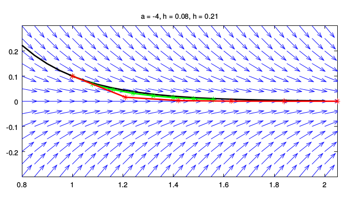
A simple model example

linear differential equation y' = a y , initial condition y(1) = 0.1

solved by explicit Euler's method using two different values of step-size h = 0.08 and h = 0.21

For a = -4, both choices of h give stable result; smaller step (green line) leads to higher accuracy than larger step (red line). Exact solution is represented by black line:

.

For a = -10 the larger step leads to instability of the explicit method:

.

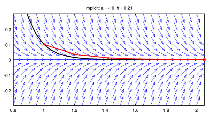
Stability of implicit Euler's method

However, the implicit Euler's method for a = -10 and larger step h = 0.21 is stable:

.

Matlab programs

All figures were created by the following two programs in Matlab (you can experiment with your own choices of parameters a and h):

%%%%%%%%%%%%%%%%%%%%%%%%%%%%%%%%%%%%%%%%%
% stability of explicit Euler's method
%%%%%%%%%%%%%%%%%%%%%%%%%%%%%%%%%%%%%%%%%

a = -10;                    % coeff. of the linear differential eq. 

h = 0.05;                   % step-size of the mesh
xh = 0.8 : h : 2 ;          % interval [ 0.8 , 2.5 ] divided with step h
yh = -0.3 : h : 0.3 ;       % interval [ 0.8 , 3.8 ] divided with step h
[xx,yy] = meshgrid(xh,yh);  % mesh on the rectangle xh, yh

  % direction field
px = ones(length(yh),length(xh));  % px = 1 at every mesh-point [x,y]
py = a*yy;                  % py = f(x,y) at every mesh-point [x,y]
pp = sqrt(px.*px + py.*py);
ppx = px./pp;               % (ppx, ppy) = normalized (px, py)
ppy = py./pp;
hold off
quiver(xh, yh, ppx, ppy)    % an arrow (ppx, ppy) at every [x,y]
hold on                    

  % exact solution
x=1; y=0.1;                 % initial condition
c = y*exp(-a*x);            % coeff. of exact solution
plot(xh, c*exp(a * xh),'LineWidth',2,'Color','k')   % exact solution


  % two numerical solutions

xp(1)=x; yp(1)=y;           % initial condition

  % smaller step
h = 0.08;           
for k=2:8
  xp(k) = xp(k-1) + h;
  yp(k) = (1 + a*h) * yp(k-1);
end
plot(xp, yp, 'g*', "markersize", 8)
plot(xp, yp, 'g','LineWidth',2)
tit = ["a = ", mat2str(a) ,", h = ", mat2str(h)]; % for the title

  % larger step
h = 0.21;    
for k=2:8
  xp(k) = xp(k-1) + h;
  yp(k) = (1 + a*h) * yp(k-1);
end
plot(xp, yp, 'r*', "markersize", 8) % , "markersize", 4
plot(xp, yp, 'r','LineWidth',2)

title([tit, ", h = ", mat2str(h)]); % title
axis([0.8, 2.05, -0.3, 0.3])  % setting a scope 
axis equal;

%%%%%%%%%%
% the end
%%%%%%%%%%


%%%%%%%%%%%%%%%%%%%%%%%%%%%%%%%%%%%%%%%%%
% stability of implicit Euler's method
%%%%%%%%%%%%%%%%%%%%%%%%%%%%%%%%%%%%%%%%%

a = -10;                    % coeff. of the linear differential eq. 

h = 0.05;                   % step-size of the mesh
xh = 0.8 : h : 2 ;          % interval [ 0.8 , 2.5 ] divided with step h
yh = -0.3 : h : 0.3 ;       % interval [ 0.8 , 3.8 ] divided with step h
[xx,yy] = meshgrid(xh,yh);  % mesh on the rectangle xh, yh

  % direction field
px = ones(length(yh),length(xh));  % px = 1 at every mesh-point [x,y]
py = a*yy;                  % py = f(x,y) at every mesh-point [x,y]
pp = sqrt(px.*px + py.*py);
ppx = px./pp;               % (ppx, ppy) = normalized (px, py)
ppy = py./pp;
hold off
quiver(xh, yh, ppx, ppy)    % an arrow (ppx, ppy) at every [x,y]
hold on                    

  % exact solution
x=1; y=0.1;                 % initial condition
c = y*exp(-a*x);            % coeff. of exact solution
plot(xh, c*exp(a * xh),'LineWidth',2,'Color','k')   % exact solution


  % numerical solution

xp(1)=x; yp(1)=y;           % initial condition

  % the larger step
h = 0.21;    
for k=2:8
  xp(k) = xp(k-1) + h;
  yp(k) = yp(k-1)/(1 - a*h) ;
end
plot(xp, yp, 'r*', "markersize", 8) % , "markersize", 4
plot(xp, yp, 'r','LineWidth',2)

tit = ["Implicit: a = ", mat2str(a) ,", h = ", mat2str(h)]; 
title(tit); % title
axis([0.8, 2.05, -0.3, 0.3])  % setting a scope 
axis equal;

%%%%%%%%%%
% the end
%%%%%%%%%%