Table of contents

• 1. Mathematical model
• 1.1. List of symbols
• 1.2. Velocity triangles for turbines and compressors
  • 1.2.1. 1.2.1 Turbine convention
  • 1.2.2. 1.2.2 Compressor convention
• 1.3. Streamline curvature method
• 1.4. Solution at the inlet section
• 1.5. Solution in free passage
• 1.6. Solution in bladed passage
• 2. Thermophysical models
• 2.1. Perfect gas
• 2.2. Aungier-Redlich-Kwong
• 3. Empirical loss and deviation models
• 3.1. Lieblein’s model
  • 3.1.1. Loss model
  • 3.1.2. Deviation model
• 3.2. Aungier’s AMDC-KO model for turbines
  • 3.2.1. Loss model
  • 3.2.2. Deviation model

1. Mathematical model

The calculation is based on the streamline curvature method. The solution is calculated in the meridional plane along the so-called quasinormals corresponding to the inlet section, leading and trailing edges, and the outlet section. The solution along a quasinormal is obtained by the solution of radial equilibrium. Effects of blade rows are included by appropriate empirical models.

1.1. List of symbols

• $C$ - the absolute velocity magnitude, in (m/s)
• $C_m$ - the meridional velocity magnitude, in (m/s)
• $C_t$ - the circumferential velocity magnitude, in (m/s)
• $W$ - the relative velocity magnitude, in (m/2), note: $C=W$ for stator
• $W_m$ - the meridional velocity magnitude, in (m/s), note $W_m=C_m$ always
• $W_t$ - the circumferential relative velocity magnitude, in (m/s)
• $p$ - the pressure, in (Pa)
• $p_{tot}$ - the total pressure, in (Pa)
• $p_{tot}'$ - the total pressure in relative system, in (Pa)
• $T$ - the temperature, in (K)
• $T_{tot}$ - the total temperature, in (K)
• $T_{tot}'$ - the relative total temperature, in (K)
• $\rho$ - the density, in (kg/s)
• $h$ - the enthalpy, in (J/kg)
• $H$ - the total enthalpy, in (J/kg)
• $H'$ - the relative total enthalpy, in (J/kg)
• $s$ - the entropy, in (J/kg/K)
• $\alpha$ - blade angles, in (deg)
• $\beta$ - flow angles, in (deg)

1.2. Velocity triangles for turbines and compressors

1.2.1. 1.2.1 Turbine convention

The orientation of angles in a turbine is follows:

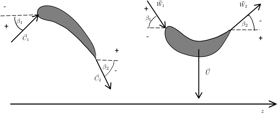
• Stator row: $W_t = C_t$
• Rotor row: $W_t = -(C_t + \omega r)$

1.2.2. 1.2.2 Compressor convention

The orientation of angles in a compressor is follows:

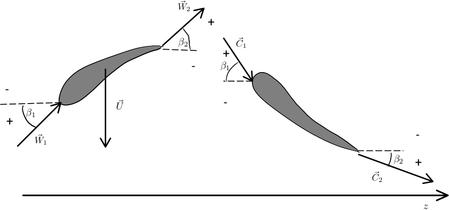
• Rotor row: $W_t = C_t + \omega r$
• Stator row: $W_t = - C_t$

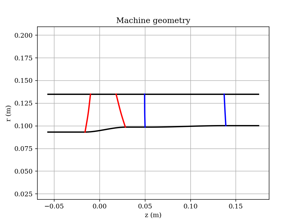
1.3. Streamline curvature method

The solution is sought in the meridional plane along quasinormals corresponding to inlet section, leading and trailing edges, and the outlet section.

The meridional view of single stage of a compressor is shown bellow. Red lines are the outlines of leading and trailing edge of rotor blades, blue lines are the leading and trailing edges of stator blades.

The computation is performed on a streamline aligned mesh shown bellow. 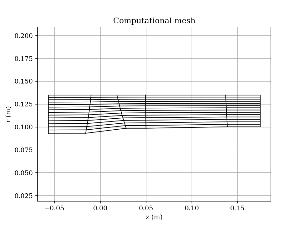The actual shape of the streamlines is obtained iteratively during the solution process.

1.4. Solution at the inlet section

The flow field at the inlet section is considered in axial direction with given total pressure, total temperature, and the mass flow rate. The inlet velocity magnitude $C_{in}$ is calculated by solving the non-linear equation $$\dot{m}_{in} = A \,\rho_{hs}(H_{tot,in} - C^2/2,s_{in}) \,C \, \cos(\varepsilon),$$ where $H_{tot,in}$ is the total enthalpy at the inlet, $s_{in}$ is the inlet entropy, and $A$ is the annulus area. The other quantities are then evaluated using thermodynamic package.

In the next step the position of streamlines at the inlet section are setup in order to keep the same amount of the mass flux between two streamlines.

1.5. Solution in free passage

The solution in a free passage between $i$ and $i+1$ quasinormal is obtained using the conservation laws: $$\begin{align*} H(i+1,j) &= H(i,j), \\ s(i+1,j) &= s(i,j), \\ C_t(i+1,j) &= C_t(i,j)\frac{r(i,j)}{r(i+1,j)} \end{align*}$$ where $j$ corresponds to streamline number.

The remaining quantities are obtained using the radial equilibrium equation. For details see e.g. Aungier

The position of streamlines along the $i+1$ quasinormal are then updated in order to keep constant amount of flux rate between two streamlines.

1.6. Solution in bladed passage

The solution at outlet edges is obtained with the help of empirical performance models. The model provides the deviation angle $\delta$ which is used for calculation of the flow angle at the outlet edge. Then, the following equations are used together with radial equilibrium: $$\begin{align*} I(i+1,j) &= I(i,j), \\ s(i+1,j) &= s(i,j) + \Delta s(i+1,j), \\ W_t(i+1,j) &= \sin(\alpha_2) C_m(i+1,j), \end{align*}$$ where $I$ is the rothalpy, $\beta_2 = \alpha_2+\delta$ is the outlet flow angle, and $\Delta s$ is the entropy increase calculated from the total pressure loss coefficient provided by the empirical model. For details see Aungier

2. Thermophysical models

2.1. Perfect gas

The perfect gas model assumes a compressible gas governed by the ideal gas equation of state $$p = \rho r T.$$ The specific heat capacity at constant pressure $c_p$ is assumed constant.

The specific enthalpy is calculated as $$h = c_p T,$$ and the specific entropy as $$s = c_p \log(T) - r \log(p).$$

Sound speed is $$a = \sqrt{\gamma r T}$$ with $\gamma = c_p/(c_p - r)$.

2.2. Aungier-Redlich-Kwong

The real gas model uses Aungier’s modification of Redlich-Kwong cubic EOS together with polynomial approximation of ideal gas contribution to $c_p$.

The Aungier-Redlich-Kwong eos is $$p = \frac{rT}{v - b + c} - \frac{a}{v(v+b)T_r^n}$$ where

• $v = 1/\rho$ is the specific volume,
• $T_r=T/T_c$ is a reduced temperature,
• $\omega$ is the user specified accentric factor,
• $a = 0.42747r^2T_c^2/p_c$,
• $b = 0.0664 r T_c/p_c$,
• $n = 0.4986 + 1.1735\omega + 0.4754\omega^2$,
• $c$ is calculated from EOS at the critical point,
• $T_c,\,v_c,\,p_c$ are the critical temperature, volume, and pressure.

The ideal gas of $c_p$ is given as a polynomial of temperature $T$: $$c_p^0(T) = \sum_{j=0}^m a_j T^j.$$

Then, the ideal gas contribution of enthalpy and entropy are $$\begin{align*} h^0(T) &= h^0_0 + \sum_{j=0}^m \frac{a_j}{j+1} T^{j+1}, \\ s_0(p,T) &= s^0_0 -r \log(p) + a_0 \log(T) + \sum_{j=1}^{m} \frac{a_j}{j}T^j, \end{align*}$$ Integration constants $h^0_0$ and $s^0_0$ are chosen in such way that the values of enthalpy and entropy (including real gas contribution, see bellow) match the values at given reference state.

The real gas contribution (departure functions) are $$\begin{align*} c_p^{r}(p,T) &= p\left(\frac{\partial v}{\partial T}\right)_p - r + \frac{\alpha(T)}{b} \frac{n (n+1)}{T} \log\left(\frac{v+b}{v}\right) + \alpha(T)(n+1)\left(\frac{\partial v}{\partial T}\right)_p \frac{1}{v(v+b)}, \\ h^r(p,T) &= p v - rT - \frac{a}{b}(n + 1)Tr^{-n}\log\left(\frac{v + b}{v}\right), \\ s^r(p,T) &= - r\log(T) + r\log(v - b + c) - \frac{n\alpha(T)}{bT}\log\left(\frac{v + b}{v}\right) + r\log(p). \end{align*}$$ where $\alpha(T)=aT_r^{-n}$.

The value of $c_p$, $h$, and $s$ is then $$\begin{align*} c_p(p,T) &= c_p^0(T) + c_p^r(p,T), \\ h(p,T) &= h^0(T) + h^r(p,T), \\ s(p,T) &= s^0(p,T) + s^r(p,T). \end{align*}$$

3. Empirical loss and deviation models

The loss and deviation model uses compressor nomenclature depicted in the following figure.

Here:

• $\beta_{1g}$ is the geometrical angle at the inlet edge (in degrees)
• $\beta_{2g}$ is the geometrical angle at the outlet edge (in degrees)
• $\beta_{1}$ is the flow angle at the inlet edge (in degrees)
• $\beta_{2}$ is the flow angle at the outlet edge (in degrees)
• $\gamma$ is the stagger angle (in degrees)
• $c$ is the blade chord
• $s$ is the cascade stagger

These quantities define following parameters:

• $i = \beta_1 - \beta_{1g}$ - the incidence angle (in degrees)
• $\delta = \beta_2 - \beta_{2g}$ - the deviation angle (in degrees)
• $\sigma = c/s$ - the cascade solidity
• $\theta = \beta_{1g} - \beta_{2g}$ blade camber angle (in degrees)

3.1. Lieblein’s model

Lieblien’s model is implemented according to

AUNGIER, Ronald H. Axial-flow compressors : a strategy for aerodynamic design and analysis. B.m.: ASME Press, 2003. ISBN 9780791801925.

The model is originally developed for compressor cascades with NACA 65 profiles.

3.1.1. Loss model

Lieblein’s loss model calculates the design incidence angle as $$i^* = K_{sh}K_{ti} \left(i^*_0\right)_{10} + n \theta$$ where $K_{sh}$ is the shape factor ($K_{sh}=1$ for NACA 65 profiles), $K_{ti}$ is the blade thickness correction, $i_0^*$ is the zero camber incidence, and $n$ is the slope factor. These parameters are calculated as $$i_0^* = \frac{\beta_{1lim}^p}{5 + 46\exp(-2.3\sigma)} - 0.1\sigma^3\exp\left((\beta_{1lim} - 70)/4\right),$$ $$p = 0.914 + \sigma^3/160,$$ $$n = 0.025\sigma - 0.06 - \frac{(\beta_{1lim}/90)^{1 + 1.2\sigma}}{1.5 + 0.43\sigma},$$ $$K_{ti} = (10t/c)^{\frac{0.28}{0.1+(t/c)^{0.3}}}.$$

The design total pressure loss is $$\omega^* = \frac{2\sigma}{\beta_2^*} \left(\frac{W_2^*}{W_1^*}\right)^2 f(D_{eq}^*),$$ where $W_{1}^* = W_{m1}/\cos(\beta_1^*)$, $W_{2}^* = W_{m2}/\cos(\beta_2^*)$, and $$f(D_{eq}^*) = K_1\left(K_2 + 3.1(D_{eq}^* - 1)^2 + 0.4(D_{eq}^* - 1)^8\right)$$ with $K_1=0.004$ and $K_2=1$ for NACA 65 profiles. The equivalent diffusion factor is defined as $$D_{eq}^* = \left(\frac{W_1^*}{W_2^*}\right) \left( 1.12 + 0.61\frac{\cos^2(\beta_1^*)}{\sigma}\left(\tan(\beta_1^*) - \tan(\beta_2^*)\right) \right).$$

The off-design loss model is then corrected for incidence angle and Mach number effects, see Aungier’s book, chapter 6.

3.1.2. Deviation model

The design deviation model has the form $$\delta^* = K_{sh} K_{t\delta} (\delta_0^*)_{10} + m \theta$$ where $K_{sh}$ is the shape factor same as for the design incidence model, $K_{t,\delta}$ is the thickness correction, $m$ is the slope parameter, and $(\delta_0^*)_{10}$ is the zero camber deviation.

According to Aungier’s book, the parameters are calculated as $$\delta_0^* = 0.01 \sigma \beta_{1lim} + \left(0.74\sigma^{1.9} + 3\sigma\right)\left(\frac{\beta_{1lim}}{90}\right)^{1.67 + 1.09\sigma}$$ where $\beta_{1lim} = \max(\min(\beta_1,70), 0)$, $$K_{t\delta} = 6.25 \frac{t}{c} + 37.5\left(\frac{t}{c}\right)^2$$

$$m = m_1 / \sigma^b$$ $$b = 0.9625 - 0.17x - 0.85x^3$$ $$m_1 = 0.17 - 0.0333x + 0.333x^2$$ with $x=\beta_{1lim}/100$.

Note that the correlation for $m_1$ depends on the profile family and the presented correlation is for NACA 65 family. Therefore $m_1$ can be configured in the input file.

The off-design correlation is then $$\delta = \delta^* + \left(\frac{\partial\delta}{\partial i}\right)^* (i - i^*) + 10\left(1 - W_{m2}/W_{m1}\right)$$ where $$\left(\frac{\partial\delta}{\partial i}\right)^* = \left(1 + (\sigma + 0.25\sigma^4)/(\beta_{1lim}/53)^{2.5}\right)\exp(-3.1\sigma)$$

3.2. Aungier’s AMDC-KO model for turbines

The outlet geometric angle corresponds to throat by pitch ratio, i.e. $\cos(\beta_{2g}) = o/s$.

3.2.1. Loss model

Total pressure loss in turbine cascade is defined as $$\begin{equation} Y = \frac{p_{tot,1}' - p_{tot,2}'}{p_{tot,1}' - p_2}. \end{equation}$$

The current version supports only the model of profile losses and losses caused by the non-zero thickness of the trailing edge, hence $$\begin{equation} Y = Y_p + Y_{TE}. \end{equation}$$

The model for profile loss is $$\begin{equation} Y_p = K_{mod} K_{inc} K_M K_p K_{Re} \left\{\left[ Y_{p1} + \zeta^2(Y_{p2} - Y_{p1})\right](5 t_{max}/c)^\zeta - \Delta Y_{TE}\right\}. \end{equation}$$ for details see Aungier.

The trailing edge loss is modeled as $$\begin{equation} Y_{TE} = \left( \frac{te}{\mathrm{pitch}\sin(\beta_2^{turb}) - te}\right)^2 \end{equation}$$ where $te$ is the trailing edge thickness.

3.2.2. Deviation model

The subsonic deviation angle for $M_2<0.5$ is calculated as $$\delta_0 = \arcsin\left[(o/s)\left(1 + (1-o/s)(\beta_{2g}^{turb}/90^\circ \right)\right] - \beta_{2g}^{turb}.$$

The deviation for for $0.5 < M_2' < 1$ is calculated as $$\begin{equation} \delta = \delta_0 \left[1 - 10 X^3 + 15 X^4 - 6 X^5\right], \end{equation}$$ with $X=2M_2' - 1$.

In the case of supersonic outlet $M_2' > 1$ the deviation follows from the conservation of mass $$\begin{equation} \delta = \arcsin\left[(o/s)\rho_*W_*/\rho_2W_2\right] - \beta_{2g}^{turb}, \end{equation}$$ where $\rho_*$ and $W_*$ are the density and velocity magnitude in the sonic point.